

You set WIP limits and they’re being ignored. Your batches are getting larger. Your lead times are getting longer. The PMO says everything’s fine.
Chapter 15 closed the safety cluster. This one returns to the work itself, where most planning still gets batch size wrong and pushes work onto teams beyond their sustainable capacity.
🎧 Prefer to listen? This chapter is narrated in my own voice with ElevenLabs on Spotify (17 minutes).
Chapter 4 asked whether the system was busy or moving. This axis asks how work is sized and routed, one level down in the same system.
The two poles
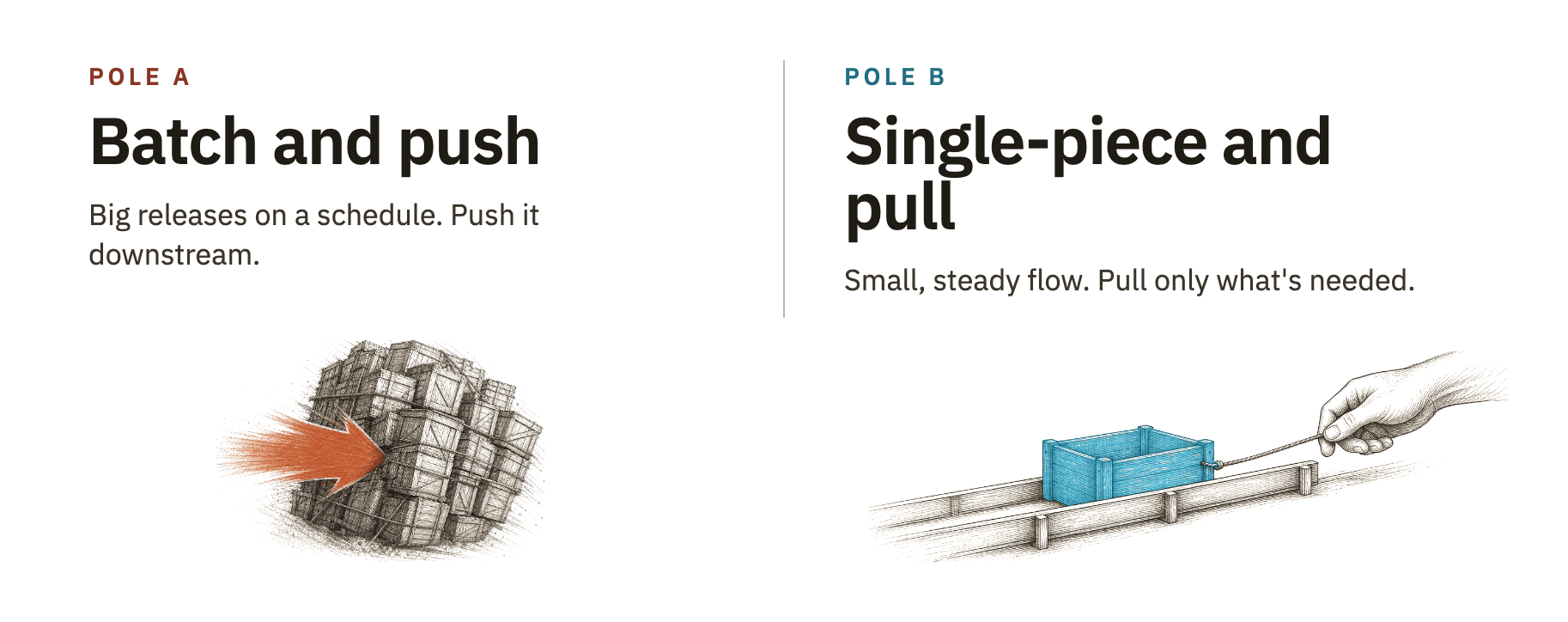
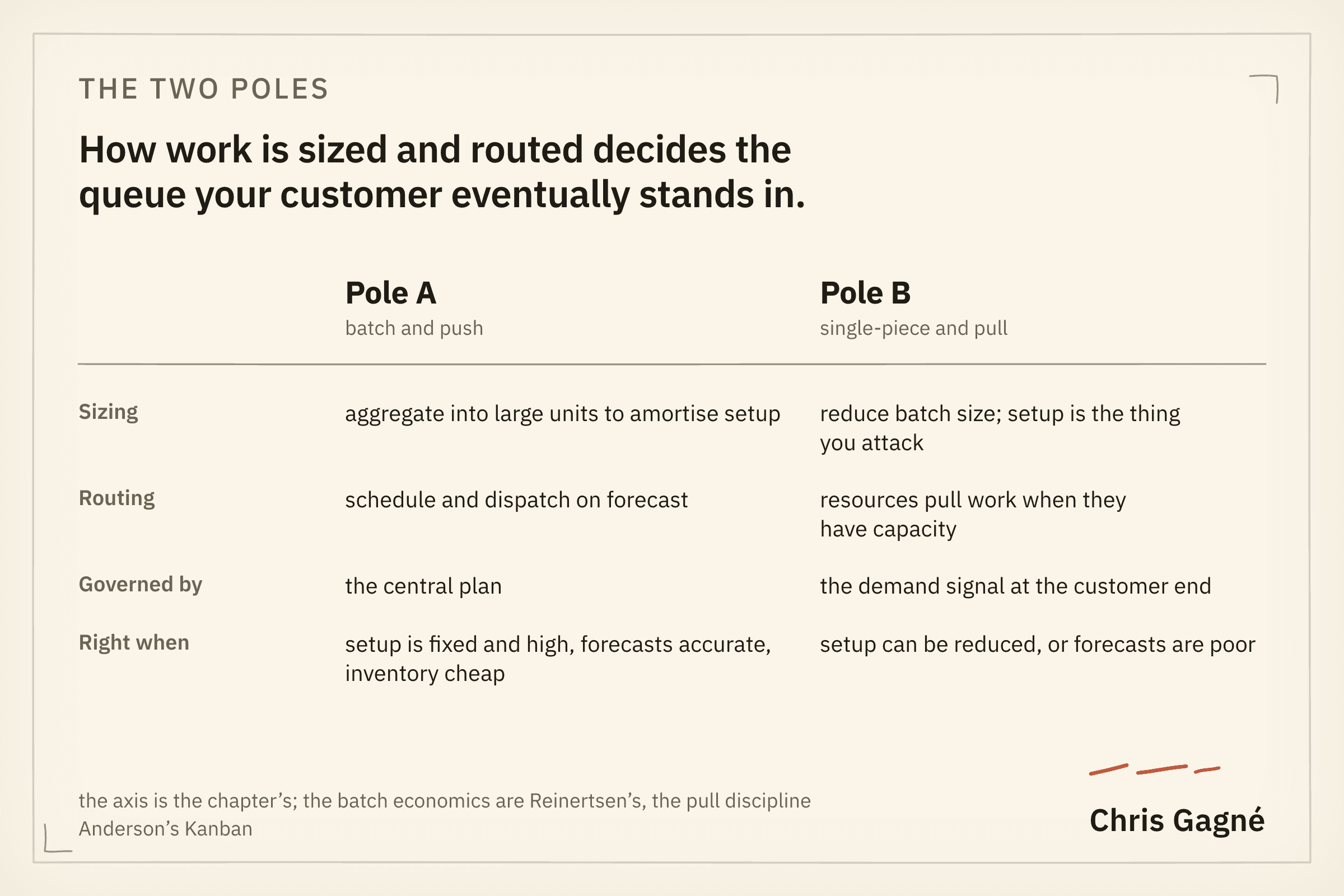
Pole A: batch and push. Aggregate work into larger units to amortise setup costs. Schedule and dispatch work to resources based on forecast. A central plan governs.
Pole B: single-piece and pull. Reduce batch size. Resources pull work when they have capacity. Demand signal at the customer end governs upstream.
Batch size and push-versus-pull are two separate levers. Batch size is how much work travels together, and it operates at three levels: the commitment horizon the board signs off, the size of a work item entering the team, and the size of a change reaching production. Push versus pull asks what triggers the next piece of work, a forecast schedule or free capacity downstream. WIP limits are the control that exposes both. The poles name the correlated ends of those levers rather than a single dial.
Where Pole A is right
When setup costs are genuinely fixed and high, demand is predictable, and inventory is cheap to hold: classical Economic Order Quantity (EOQ) logic in mature physical operations. The 1913 model assumes fixed setup and predictable demand, and prices the cost of holding inventory as an input. Raise that input and the model itself calls for a smaller batch. In the small slice of contemporary work that still meets them, the Pole A maths holds.
A pharmaceutical manufacturing line with a multi-hour changeover and a regulated batch certification has fixed setup costs the operator can’t reduce. A semiconductor fab with a stable product mix has forecast accuracy a software team can’t match. The EOQ logic in those settings is sound maths. The planning most engineering organisations inherited was built for those settings, and the leaders who built it weren’t wrong about the world they built it for.
Where Pole B is right
Pole B is right wherever setup costs can themselves be reduced and the learning rate matters, where forecast accuracy is low, variation is high, and the holding cost of inventory is high. A deploy whose entire changeover is a CI run measured in minutes sits at the opposite end from the pharma line above. Software work with reducible setup cost, uncertain demand, or costly ageing inventory tends toward smaller batches.
In decisions
Pole A leaders schedule long roadmaps—queues if we are willing to use a more truthful name—and allocate capacity with long planning intervals. Pole B leaders ship continuously, set WIP limits, and let teams pull from a prioritised and pruned backlog.
The batch-versus-pull axis is set by the planning the CEO runs with the board, and that is the conversation a CTO or VPE has to take upward. If the CEO commits to a quarterly or yearly roadmap with the board, the engineering organisation is pushed to batch work into large commitments no matter what the team-level discipline says.
Put two measures in front of them: the cost of delay on one current initiative, in the CEO’s unit of account, and the change in cycle time the team achieved when WIP limits were last set and held. If you have never held one, the exercise at the end of this chapter produces that number in a sprint. Don’t turn this into an Agile lesson. Show the downstream cost: the planning they use with the board propagates into batch sizes the company and customer eventually pay for.
Then ask for one change. What the board wants is confidence about risk and return; a 12-month feature list is a proxy for that, and a poor one, since I’ve never seen one delivered as written. OpenAI and Anthropic commit billions of dollars in compute years ahead and publish no dated feature roadmap. They commit capacity and direction, and refuse to commit the sequence. An incumbent with contracts and regulators can’t copy that outright, and doesn’t need to. Start with a count. How much of the roadmap is genuinely contracted, and how much is merely scheduled? In the organisations I see, the contracted share is small, and the rest had been treated as fixed anyway. Ask to take delivery rate and a record of what you redirected and why to the board instead.
The sentence your CEO can carry to the board: “The planning calendar we run with the board becomes the queue our pending value stands in.”
The planning calendar we run with the board becomes the queue our pending value stands in.
The EOQ trap
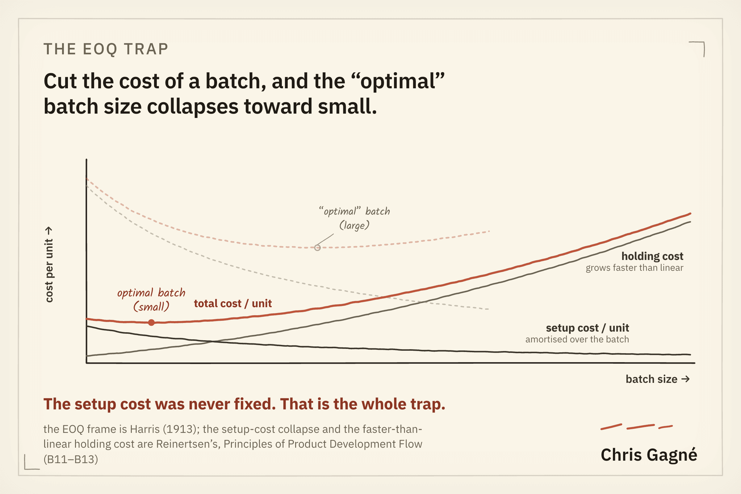
I suspect the Economic Order Quantity model is the least examined planning artefact in operations, and part of the reason is that almost nobody in software names it. The logic arrives second-hand, built into the planning calendar and the release train, and an assumption nobody names is one nobody audits. The 1913 model assumes fixed setup costs (which means setup reduction can’t change the result), accurate demand forecasts (which means uncertainty is small), and a holding cost that rises in a straight line with the batch (which means a big batch costs only proportionately more to hold). It then derives an optimal batch size from those assumptions.
The maths is correct. Reinertsen’s own demolition runs through the cost legs: the “fixed” transaction cost isn’t fixed (Japanese manufacturers cut die changeovers from 24 hours to under ten minutes, using the single-minute exchange of dies (SMED) methods Shigeo Shingo pioneered), transaction costs actually grow with batch size, and holding costs grow faster than linearly.
The trouble starts when one input no longer holds. If setup costs can be reduced—through tooling, automation, practice—the optimal batch size collapses. Low forecast accuracy does the same because the cost of being wrong about a large batch is much higher than about a small one. So does high inventory holding cost, especially when inventory has a short shelf life or hides quality problems. Setup cost is structural as much as technical. A method that convenes a two-day planning event for a whole programme every quarter carries a far higher transaction cost per batch than one that plans in a few hours each sprint. Hyper-specialisation compounds it. When every department is optimised on its own, finishing anything means crossing more of them, and each crossing adds coordination the batch has to carry. The dependencies raise the transaction cost, and the higher transaction cost argues for the bigger batch.
Of the three, the setup-cost leg is moving fastest right now. AI-assisted engineering cuts the cost of producing and testing a change, which moves the optimum down the same way SMED did. My hunch is that it also moves the constraint, toward review, integration, and the demand governance deciding what gets built at all, none of which got faster at the same rate. If that holds, the WIP limit belongs where the work now waits: on review and integration, not on authoring. Don’t author faster than you can review and integrate.
The fact that the planning still defaults to legacy EOQ-shaped logic—large batches, long forecasts, central planning—is doctrinal lag. The maths says one thing; the org chart says another; the doctrine sided with the org chart. The critique predates Agile and DevOps: Goldratt’s The Goal ran it in narrative form in 1984, halving batch sizes against the economic-batch-quantity doctrine. Reinertsen supplies the general mathematics.
Reinertsen on batch-size economics
Donald Reinertsen‘s The Principles of Product Development Flow gives the maths at industrial scale. It spells out how batch size, queues, and economic cost of delay lock together, with a precision the fragments of Lean and Agile most leaders inherit leave out.
Batch size moves five variables at once: as batches shrink, cycle time, queue size, and risk fall while feedback rate and learning rise. The cost of reducing batch size—usually some setup-cost-per-batch—has to be weighed against the compounding benefit.
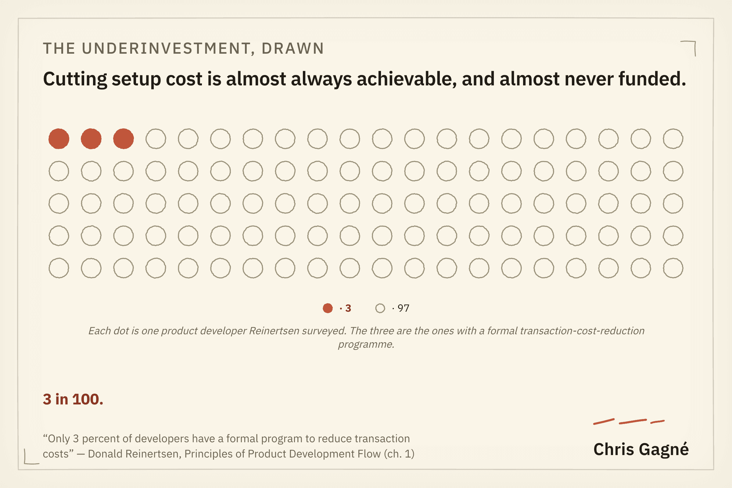
Reinertsen’s running diagnostic comes from his own surveys of product developers, only 3% of whom had a formal transaction-cost-reduction programme. The cost-of-setup reduction is almost always achievable and almost always underinvested. It stays underinvested as a matter of inherited default, not because the economics favour the old batch size. Cheap switching is what makes adaptiveness affordable. The test is simple: after fresh evidence arrived, did the next item pulled actually change? A team can hold a hard WIP limit against a backlog nobody has touched in a year, and all the discipline buys is faster delivery of a stale plan.
Reinertsen’s cost of delay, the economic argument chapter 4 made in full, applies directly to batch size. The visible cost (an engineer’s idle hour) wins planning conversations by default; the invisible cost, the delay a deep queue causes, never shows up until someone dollarises it.
Anderson’s kanban
David Anderson’s Kanban names the operational discipline. Anderson asks teams to make workflow visible, cap work in progress, measure and manage flow, state process policies aloud, and use explicit models to find where to improve. The board is the truth; the plan is the hypothesis.
The failure I meet most often is treating kanban as a visualisation layer rather than a discipline. You adopt the board, the WIP limits get ignored, batches keep entering above the system’s capacity, and the conclusion is that kanban doesn’t fit your kind of work. When items keep entering above the cap, the board is serving as a status display rather than flow control. The WIP limit is the operative constraint. The board makes the constraint visible.
The operating system
Follow one item through. It is pulled when a slot opens rather than pushed when someone plans it, so it moves without waiting behind a batch. It ships small enough that the team learns something within days rather than at the end of a quarter. What they learn changes how the next one is pulled. Gene Kim’s DevOps Handbook names those three motions the Three Ways: Flow, Feedback, and Continual Learning. The first two you can build. The third is what the org design either permits or prevents, and it is what keeps the other two from eroding.
In the State of DevOps data the fastest-deploying organisations, deploying on demand many times a day, also carry the lowest change-failure rates. The Pole A intuition that fast deployment is reckless is inverted by the measurement. Small change size is the likeliest mechanism—less can go wrong in a five-line change than in a 500-line one—though the surveys measure association rather than cause.
A representative case
The version I ran started somewhere less tidy than a planning problem. Demand was arriving well above delivery capacity. When we read queue length as time-to-clear at the observed rate, the answers came back in months and years. Nobody had been lying about the roadmap. The arithmetic had simply never been done out loud.
Three changes.
First, make the queue visible in time rather than in items. A count of stories is a number; most of a year to clear at the current rate is a decision.
Second, put a hard edge on intake. Work went into two lanes with a stated order, and a displacement rule: when incoming unplanned work would push an iteration past the team’s raw velocity, enough planned work had to come out, with a comment on both stories recording what changed and why. The trade stopped being invisible.
Third, set a work-in-process threshold and let it stop the line. More than 1.3 stories per builder, or more than three-quarters of an iteration’s worth in process, and intake froze. Both numbers were starting defaults, open to revision in retrospective, and they got argued about, which was the point: arguing about the threshold is arguing about capacity.
The diagnostic move
Three questions for last sprint’s allocation:
- Which pole was I claiming? Did I describe the work as batched-and-pushed or single-piece-and-pulled?
- Which pole would the actual batch sizes show? If I measured the average size of work items entering the system, would it look like Pole A or Pole B?
- Which pole does this work actually require? EOQ wants a fixed setup cost, demand you can treat as known, and a holding cost that rises in a straight line. Miss any of those and the economic batch size drops. How far is a question for measurement, not doctrine.
The exercise
Run a WIP-limit experiment for one sprint. Set a hard team-wide WIP limit: say four items in progress total or half a sprint’s velocity, not per person. Pull from a ruthlessly pruned backlog. Measure lead time and cycle time before and after. The exercise produces three useful surprises. The team finds out which items have been passively blocked: sitting in progress because nobody had to kill them. The team feels how unfamiliar it is to pull rather than push. And the leader gets a clear lead-time signal that no roadmap-status conversation produces.
A second variant for teams already running kanban: run a kata cycle on one constraint. Pick the stage where work piles up, name a target condition (how that stage should operate to produce a specific cycle time), identify the next obstacle, run a small experiment, learn, repeat weekly. Run the Toyota improvement kata as a four-week experiment.
Going upstream
Watch. Henrik Kniberg, High WIP, Context Switching vs One Piece Flow (Vimeo, 7 min). Don Reinertsen, GOTO 2012 Interview on flow (24 min). Companion short hook: Reinertsen, Economics of Batch Size and the “Father-Egg” Story (4 min).
In-text: The two main sources named in the chapter. Don Reinertsen, The Principles of Product Development Flow (the Q-series, E-series, and B-series principles together, including batch-size economics and the EOQ demolition). David J. Anderson, Kanban (the WIP-limit discipline behind the exercise).
Also touched: Eli Goldratt, The Goal, for the 1984 batch-halving antecedent to the EOQ critique (worked at full length in the local-optima instalment). Gene Kim et al., The DevOps Handbook (Chapter 1 on the Three Ways), the structure that lets Reinertsen and Anderson compose into one operating system.
Go deeper: The lineage that names the same single-piece discipline at different layers, demoted here and carried elsewhere in the book. Mary and Tom Poppendieck, Lean Software Development (the seven principles for translating lean to software: cutting waste, building in learning, deferring commitment, shipping quickly, giving teams authority, designing quality in from the start, and optimising the whole rather than the parts) and The Lean Mindset, for the Toyota-Production-System-to-software translation. Jez Humble and David Farley, Continuous Delivery, for the deployment pipeline that makes large batches structurally expensive (developed in the utilisation-versus-flow instalment). Kent Beck, Extreme Programming Explained, for embrace change and the short-cycle cultural discipline. Mike Rother, Toyota Kata, for the coaching and improvement kata behind the exercise variant; the constraint-first selection above is the Goldratt overlay, since Rother starts from the pacemaker process, and he is precise that a number alone is a target, not a target condition. Gene Kim et al., The Phoenix Project, for the narrative form. Nicole Forsgren, Jez Humble, Gene Kim, Accelerate, the State of DevOps reports across four years, for the empirical correlation: high software-delivery performers are twice as likely as low performers to exceed profitability, productivity, and market-share goals, and the fastest-deploying organisations carry the lowest change-failure rates.
I work with engineering leaders on exactly this kind of paradigm work, the deeper the better. If it’s live for you, I’m happy to talk: schedule a 30-minute virtual coffee at hi.chrisgagne.com.
Some book links here are Amazon affiliate links; if you buy through them I may earn a small commission, at no cost to you.
Small batches and pull only move work if someone holds the authority to decide what gets pulled, and in most structures that person is you. The queue forms on your calendar. Tuesday fills with approvals, the team stalls on any decision you haven’t signed, and the function gains no speed for all the oversight. You are the bottleneck. Chapter 17 names the default that put you there, leader-follower, and sets David Marquet’s leader-leader against it.
Leave A Comment